Here we introduce the cylindrical coordinate system for vector fields to describe axisymmetric flows, and derive the expressions of classical differential operators in cylindrical coordinates.
Coordinate transform
Denote the standard basis as $e_1,e_2,e_3$ and $x_1,x_2,x_3$ the coordinate in $\R^3$. Let
$$(r,\theta,h)=\br{\sqrt{x_1^2+x_2^2}, \arctan \br{\frac {x_2}{x_1} },x_3}\Longleftrightarrow (x_1,x_2,x_3)=(r\cos \theta, r\sin \theta,h).$$This induce the Jacobi matrix between $(x_1,x_2,x_3)\sim (r,\theta,z)$ and its inverse
\begin{equation*}
J\eqqcolon
\begin{pmatrix}
\dfrac{\partial r }{\partial x_1 } & \dfrac{\partial r }{\partial x_2 } & \dfrac{\partial r }{\partial x_3 }\\
\dfrac{\partial \theta }{\partial x_1 } & \dfrac{\partial \theta }{\partial x_2 } & \dfrac{\partial \theta }{\partial x_3 } \\
\dfrac{\partial h }{\partial x_1 } & \dfrac{\partial h }{\partial x_2 } & \dfrac{\partial h }{\partial x_3 } \\
\end{pmatrix}
=
\begin{pmatrix}
\cos \theta & \sin\theta & 0 \\
-\dfrac{\sin \theta }{r} & \dfrac{\cos \theta }{r} & 0\\
0 & 0 & 1
\end{pmatrix} \Longleftrightarrow J^{-1}=
\begin{pmatrix}
\dfrac{\partial x_1 }{\partial r } & \dfrac{\partial x_1 }{\partial \theta } & \dfrac{\partial x_1 }{\partial h } \\
\dfrac{\partial x_2 }{\partial r } & \dfrac{\partial x_2 }{\partial \theta } & \dfrac{\partial x_2 }{\partial h } \\
\dfrac{\partial x_3 }{\partial r } & \dfrac{\partial x_3 }{\partial \theta } & \dfrac{\partial x_3 }{\partial h } \\
\end{pmatrix}=
\begin{pmatrix}
\cos \theta & -r\sin \theta & 0\\
\sin \theta & r \cos \theta & 0\\
0 & 0 & 1
\end{pmatrix}.
\end{equation*}And we choose the another orthonormal basis as
\begin{equation}
\label{cylinderical-jacobi}
\begin{pmatrix}
e_r \\ e_\theta \\ e_h
\end{pmatrix}
=\begin{pmatrix}
\cos \theta & \sin \theta & 0\\
-\sin \theta & \cos \theta & 0\\
0 & 0 &1\\
\end{pmatrix}
\begin{pmatrix}
e_1\\ e_2\\ e_3
\end{pmatrix}
\Longleftrightarrow \begin{pmatrix}
e_1 \\ e_2 \\ e_3
\end{pmatrix}
=\begin{pmatrix}
\cos \theta & -\sin \theta & 0\\
\sin \theta & \cos \theta & 0\\
0 & 0 & 1\\
\end{pmatrix}
\begin{pmatrix}
e_r\\ e_\theta\\ e_h
\end{pmatrix}.
\end{equation}The physical correspondence can be interpreted by the following graph:
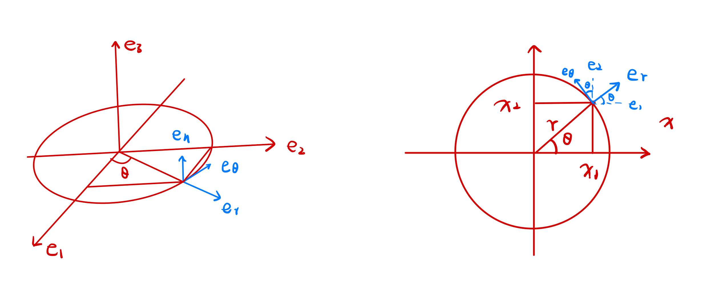
A significant fact is that the cylindrical coordinate does not stay stationary. Indeed, we can compute the cylindrical derivative of the basis using the above Jacobi matrix \eqref{cylinderical-jacobi}:
\begin{equation}
\begin{split}
\partial_\theta e_r =& \partial_\theta (\cos \theta e_1+\sin \theta e_2 )=-\sin \theta e_1+\cos \theta e_2 =e_\theta, \\
\partial_\theta e_\theta= &\partial_\theta (-\sin \theta e_1+\cos \theta e_2 )= -\cos \theta e_1-\sin \theta e_2=-e_r,\\
\partial_r e_r=& \partial_r e_\theta=\partial_h e_r=\partial_h e_\theta=\partial_r e_h=\partial_\theta e_h =0= \partial_he_h=0.
\end{split}
\end{equation}Consider $v=v^1e_1+v^2e_2+v^3e_3=v^re_r+v^\theta e_\theta+v^he_h$. Under this coordinate system, the classical differential operator now has new expressions:
| Name | Symbol | Cartesian | Cylindrical |
|---|---|---|---|
| Gradient | $\nabla f$ | $(\partial_1, \partial_2, \partial_3)$ | $\br{\partial_r , \frac 1r \partial_\theta, \partial_h }$ |
| Skew gradient | $\nabla^\perp f$ | $(-\partial_2, \partial_1 )$ | $\br{-\frac 1r \partial_\theta , \partial_r }$ |
| Divergence | $\div f= \nabla \cdot f$ | $\partial_1 v^1+\partial_2 v^2+\partial_3 v^3$ | $\frac 1{r} {\partial_r(rv^r) }+\frac 1r \partial_\theta v^\theta +\partial_h v^h$ |
| Curl | $\curl f= \nabla \times f$ | $\begin{pmatrix}\partial_2 v^3-\partial_3 v^2\\\partial_3 v^1-\partial_1 v^3\\\partial_1 v^2-\partial_2 v^1 \end{pmatrix}$ | $\begin{pmatrix}\frac 1r \partial_\theta v^h-\partial_h v^\theta \\\partial_h v^r-\partial_r v^h\\\frac 1r\br{\partial_r (rv^\theta) -\partial_\theta v^r}\\\end{pmatrix}$ |
| Material derivative | $D_t=\partial_t + u\cdot \nabla$ | $\partial_t+ u^1 \partial_1 +u^2 \partial_2+u^3 \partial_3$ | $\partial_t +u^r \partial_r +\frac 1r u^\theta \partial_\theta +u^h \partial_h$ |
| Laplacian | $\Delta f$ | $\partial_1^2 f+\partial_2^2 f+\partial_3^2 f$ | $\frac 1r\partial_r \br{r \partial_r f}+\frac 1{r^2}\partial_\theta^2 f+\partial_h^2f$ |
| Vector Laplacian | $\Delta v$ | $(\Delta v^1,\Delta v^2,\Delta v^3 )$ | $\begin{pmatrix}\Delta v^r-\frac{1}{r^2}v^r-\frac{2 }{r^2}\partial_\theta v^\theta\\\Delta v^\theta -\frac{v^\theta}{r^2}+\frac{2\partial_\theta v^r}{r^2} \\\Delta v^h\end{pmatrix}$ |
Gradient
Consider the gradient operator $\nabla =e_1\partial_1 +e_2\partial_2 +e_3\partial_3 =e_r\partial_r +e_\theta\dfrac 1r \partial_\theta +e_h\partial_h $:
\begin{equation*}
\begin{split}
\nabla = & \br{e_1,e_2,e_3}\begin{pmatrix}
\partial_1 \\ \partial_2\\ \partial_3
\end{pmatrix}
= (e_r, e_\theta, e_h)
\begin{pmatrix}
\cos \theta & \sin \theta & 0\\
-\sin \theta & \cos \theta & 0\\
0 & 0 & 1\\
\end{pmatrix}
\begin{pmatrix}
\cos \theta & -\dfrac{\sin \theta }{r} & 0 \\
\sin\theta & \dfrac{\cos \theta }{r} & 0\\
0 & 0 & 1
\end{pmatrix}
\begin{pmatrix}
\partial_r \\ \partial_\theta\\ \partial_h
\end{pmatrix}\\
=& (e_r, e_\theta, e_h)
\begin{pmatrix}
1 & 0 & 0 \\
0 & \dfrac 1r & 0 \\
0 & 0 & 1\\
\end{pmatrix}
\begin{pmatrix}
\partial_r \\ \partial_\theta\\ \partial_h
\end{pmatrix}= e_r\partial_r +e_\theta\dfrac 1r \partial_\theta +e_h\partial_h .
\end{split}
\end{equation*}
Skew gradient
Skew gradient operator $\nabla^\perp$ represent a counterclock $\frac \pi 2-$rotation of the gradient operator in 2D case. In the standard coordinate, we have $\nabla^\perp =-e_1 \partial_2 +e_2\partial_1=(-\partial_2,\partial_1 ) $. When it turns to the 2D cylindrical coordinate, we can compute directly from the Jacobi matrix:
\begin{equation*}
\begin{split}
\nabla^\perp =&\begin{pmatrix}
e_1 & e_2
\end{pmatrix}
\begin{pmatrix}
-\partial_2\\
\partial_1
\end{pmatrix}
=\begin{pmatrix}
e_1 & e_2
\end{pmatrix}
\begin{pmatrix}
0 & -1\\
1 & 0
\end{pmatrix}
\begin{pmatrix}
\partial_1\\
\partial_2
\end{pmatrix}\\
=&\begin{pmatrix}
e_r & e_\theta
\end{pmatrix}
\begin{pmatrix}
\cos \theta & \sin \theta \\
-\sin \theta & \cos \theta
\end{pmatrix}
\begin{pmatrix}
0 & -1\\
1 & 0
\end{pmatrix}
\begin{pmatrix}
\cos \theta & -\dfrac{\sin \theta }{r} \\
\sin\theta & \dfrac{\cos \theta }{r} \\
\end{pmatrix}
\begin{pmatrix}
\partial_r\\
\partial_\theta
\end{pmatrix}\\
=& e_r\br{-\frac 1r \partial_\theta}+e_\theta \partial_r.
\end{split}
\end{equation*}The skew gradient can also be recovered from the curl operator, where you can see details in the relative part.
Divergence
Divergence operator $\div v=\nabla \cdot v $. We apply the Leibniz rule to derive
\begin{equation*}
\begin{split}
\div v=& \nabla \cdot (v^r e_r+v^\theta e_\theta +v^h e_h )\\
=& (\nabla v^r )\cdot e_r +(\nabla v^\theta )\cdot e_\theta+ (\nabla v^h )\cdot e_h\\
&+v^r(\nabla \cdot e_r )+v^\theta (\nabla \cdot e_\theta )+v^h(\nabla\cdot e_h )\\
\end{split}
\end{equation*} Here we use the chain rule to compute
\begin{equation*}
\begin{split}
\nabla \cdot e_r=&e_r \cdot \partial_r e_r +e_\theta \cdot \frac 1r \partial_\theta e_r+e_h \cdot \partial_h e_r=e_\theta \cdot \frac 1r e_\theta=\frac 1r ,\\
\nabla \cdot e_\theta=& e_r \cdot \partial_r e_\theta +e_\theta \cdot \frac 1r \partial_\theta e_\theta+e_h \cdot \partial_h e_\theta=e_\theta \cdot \br{-\frac 1r e_r}=0,\\
\nabla \cdot e_h=& e_r \cdot \partial_r e_h +e_\theta \cdot \frac 1r \partial_\theta e_h+e_h \cdot \partial_h e_h=0.
\end{split}
\end{equation*} Consequently,
\begin{equation*}
\div v=\partial_r v^r+\frac 1r \partial_\theta v^\theta +\partial_h v^h+ \frac {v_r}{r}=\frac {\partial_r(rv^r) }{r}+\frac 1r \partial_\theta v^\theta +\partial_h v^h.
\end{equation*}
Curl
Curl operator $\curl v=\nabla \times v$. The derivation is similar with the above:
\begin{equation*}
\begin{split}
\curl v=& \nabla \times \br{v^r e_r+v^\theta e_\theta+ v^he_h }\\
=& (\nabla v^r)\times e_r +(\nabla v^\theta )\times e_\theta+ (\nabla v^h )\times e_h\\
&+v^r(\nabla \times e_r )+v^\theta (\nabla \times e_\theta )+v^h (\nabla \times e_h).
\end{split}
\end{equation*} Here $e_r\times e_\theta=e_h, e_\theta\times e_h=e_r, e_h\times e_r =e_\theta $, and
\begin{equation*}
\begin{split}
\nabla \times e_r=& e_r \times \partial_r e_r +e_\theta \times \frac 1r \partial_\theta e_r +e_h \times \partial_h e_r=e_\theta \times \frac 1r e_\theta=0,\\
\nabla \times e_\theta=& e_r \times \partial_r e_\theta +e_\theta \times \frac 1r \partial_\theta e_\theta +e_h \times \partial_h e_\theta=e_\theta \times \br{-\frac 1r e_r}=\frac 1r e_h,\\
\nabla \times e_h=& e_r \times \partial_r e_h +e_\theta \times \frac 1r \partial_\theta e_h +e_h \times \partial_h e_h=0,\\
\end{split}
\end{equation*} Combine them together, then we finally get
\begin{equation*}
\begin{split}
\curl v=& (e_r\partial_r v^r +e_\theta\dfrac 1r \partial_\theta v^r +e_h\partial_h v^r)\times e_r+(e_r\partial_r v^\theta +e_\theta\dfrac 1r \partial_\theta v^\theta+e_h\partial_h v^\theta)\times e_\theta\\
&+(e_r\partial_r v^3 +e_\theta\dfrac 1r \partial_\theta v^3+e_h\partial_h v^h)\times e_h+\frac{v^\theta }{r}e_h\\
=& \br{ -\partial_h v^\theta+\frac 1r \partial_\theta v^h }e_r+\br{\partial_h v^r-\partial_r v^h }e_\theta +\br{-\frac1r\partial_\theta v^r+\partial_r v^\theta +\frac {v^\theta}{r} } e_h\\
=& \br{ \frac 1r \partial_\theta v^h-\partial_h v^\theta }e_r+\br{\partial_h v^r-\partial_r v^h }e_\theta +\frac 1r\br{\partial_r (rv^\theta) -\partial_\theta v^r }e_h.
\end{split}
\end{equation*} Moreover, it can be written in determinant form:
\begin{equation*}
\curl v=\nabla\times v= \frac 1r \begin{vmatrix}
e_r & re_\theta & e_h\\
\partial_r & \partial_\theta & \partial_h\\
v^r & rv^\theta & v^h
\end{vmatrix}.
\end{equation*} On the other hand, the curl operator has following relation with the skew gradient:
\begin{equation*}
\nabla^\perp f=- \curl \br{0,0,f}=e_r \br{\frac 1r \partial_\theta f }+e_\theta \br{-\partial_r f}=\br{-\frac 1r \partial_\theta, \partial_r } f.
\end{equation*} And if $v$ is 2D, i.e. $v=v^r(r,\theta)e_r+v^\theta (r,\theta)e_\theta$, then
\begin{equation*}
\begin{split}
\curl v= \frac 1r \br{ \partial_r (rv^\theta )-\partial_\theta v^r }e_\theta =\br{\nabla^\perp \cdot v }e_\theta.
\end{split}
\end{equation*} These relations are used in the 2D incompressible fluids to expressible the relation of the vorticity, velocity and the stream function.
Material derivative
Material derivate $D_t = \partial_t +u\cdot \nabla$, where $u=u^re_r+u^\theta e_\theta+u^he_h$ is the velocity.
\begin{equation*}
\begin{split}
D_t = & \partial_t + (u^re_r+u^\theta e_\theta +u^h e_h )\cdot (e_r \partial_r +e_\theta \frac 1r \partial_\theta+ e_h \partial_h )\\
= & \partial_t +u^r \partial_r +\frac 1r u^\theta \partial_\theta +u^h \partial_h.
\end{split}
\end{equation*}
Laplacian
Laplace operator $\Delta=\nabla \cdot \nabla$. This need to be considered in scalar and vector case respectively. If $f$ is a scalar function, we can compute $\Delta f$ out directly from gradient and divergence operator:
\begin{equation*}
\begin{split}
\Delta f =& \frac{\partial_r (r(\partial_r f)) }{r}+\frac 1r\partial_\theta(\frac 1r \partial_\theta f)+\partial_h(\partial_h f)\\
=& \frac 1r\partial_r \br{r \partial_r f}+\frac 1{r^2}\partial_\theta^2 f+\partial_h^2f.
\end{split}
\end{equation*} If $v=v^r e_r +v^\theta e_\theta +v^h e_h$ is a vector function, then
\begin{equation*}
\begin{split}
\Delta v=& \frac 1{r^2} \br{r \partial_r}^2 (v^r e_r +v^\theta e_\theta +v^h e_h)+\frac 1{r^2}\partial_\theta^2 (v^r e_r +v^\theta e_\theta +v^h e_h)+\partial_h^2(v^r e_r +v^\theta e_\theta +v^h e_h)\\
=& \br{\frac 1{r^2} \br{r \partial_r}^2 v^r+\frac 1{r^2}\partial_\theta^2 v^r +\partial^2_h v^r } e_r +\br{\frac 1{r^2} \br{r \partial_r}^2 v^\theta+\frac 1{r^2}\partial_\theta^2 v^\theta +\partial^2_h v^\theta } e_\theta + \br{\frac 1{r^2} \br{r \partial_r}^2 v^h+\frac 1{r^2}\partial_\theta^2 v^h +\partial^2_h v^h } e_h\\
& + \frac 2{r^2} (r\partial_r v^r) (r\partial_r e_r) +\red{ \frac 2{r^2} (\partial_\theta v^r)\br{\partial_\theta e_r }}+2(\partial_h v^r )\br{ \partial_h e_r } \\
& + \frac 2{r^2} (r\partial_r v^\theta ) (r\partial_r e_\theta) +\red{\frac 2{r^2} (\partial_\theta v^\theta)\br{\partial_\theta e_\theta }}+2(\partial_h v^\theta )\br{ \partial_h e_\theta }\\
& + \frac 2{r^2} (r\partial_r v^h) (r\partial_r e_h) +\frac 2{r^2} (\partial_\theta v^h)\br{\partial_\theta e_h }+2(\partial_h v^h )\br{ \partial_h e_h }\\
& + \frac 1{r^2} v^r \br{r \partial_r }^2 e_r+\red{ \frac 1{r^2} v^r \partial_\theta^2 e_r} +v^r \partial_h^2 e_r \\
& + \frac 1{r^2} v^\theta \br{r \partial_r }^2 e_\theta+ \red{\frac 1{r^2} v^\theta \partial_\theta^2 e_\theta} +v^\theta \partial_h^2 e_\theta\\
& + \frac 1{r^2} v^h \br{r \partial_r }^2 e_h+ \frac 1{r^2} v^h \partial_\theta^2 e_h +v^h \partial_h^2 e_h \\
=& \Delta v^r e_r + \Delta v^\theta e_\theta +\Delta v^h e_h + \frac 2{r^2} (\partial_\theta v^r)e_\theta -\frac 2{r^2} (\partial_\theta v^\theta)e_r-\frac 1{r^2} v^r e_r-\frac 1{r^2} v^\theta e_\theta \\
=& \br{\Delta v^r-\frac{v^r}{r^2}-\frac{2\partial_\theta v^\theta }{r^2} }e_r+\br{\Delta v^\theta -\frac{v^\theta}{r^2}+\frac{2\partial_\theta v^r}{r^2} }e_\theta +\Delta v^h e_h.
\end{split}
\end{equation*}